elm Overview / Example

This page walks through a Jupyter notebook using elm to ensemble fit K-Means and predict from all members of the ensemble.

It demonstrates the common steps of using elm :

• Working with elm.readers.load_array to read NetCDF , HDF4 , HDF5 , and GeoTiff files, and controlling how a sample is composed of bands or separate rasters with BandSpec . See also Creating an ElmStore from File
• Defining a Pipeline of transformers (e.g. normalization and PCA) and an estimator, where the transformers use classes from elm.pipeline.steps and the estimator is a model with a fit / predict interface. See also Pipeline
• Calling fit_ensemble to train the Pipeline under varying parameters with one or more input samples
• Calling predict_many to predict from all trained ensemble members to one or more input samples

LANDSAT

The LANDSAT classification is notebook from elm-examples . This section walks through that notebook, pointing out:

• How to use elm.readers for scientific data files like GeoTiffs
• How to set up an elm.pipeline.Pipeline of transformations
• How to use dask to fit a Pipeline in ensemble and predict from many models

NOTE : To follow along, make sure you follow the Prerequisites for Examples. The LANDSAT sample used here can be found in the `AWS S3 LANDSAT bucket here`_.

elm.readers Walk-Through

First the notebook sets some environment variables related to usage of a dask-distributed Client and the path to the GeoTiff example files from elm-data:

Each GeoTiff file has 1 raster (band of LANDSAT data):

See more inforation on ElmStore in ElmStore.

elm.readers.BandSpec

Using a list of BandSpec objects, as shown below, is how one can control which bands, or individual GeoTiff files, become the sample dimensions for learning:

• buf_xsize: The size of the output raster horizontal dimension
• buf_ysize: The size of the output raster vertical dimension
• name: What do call the band in the ElmStore returned. For example band_1 as a name will mean you can use X.band_1 and find band_1 as a key in X.data_vars.
• search_key: Where to look for the band identifiying info, in this case the file name
• search_value : What string token identifies a band, e.g. B1.TIF (see file names printed above)

We are using buf_xsize and buf_ysize below to downsample.

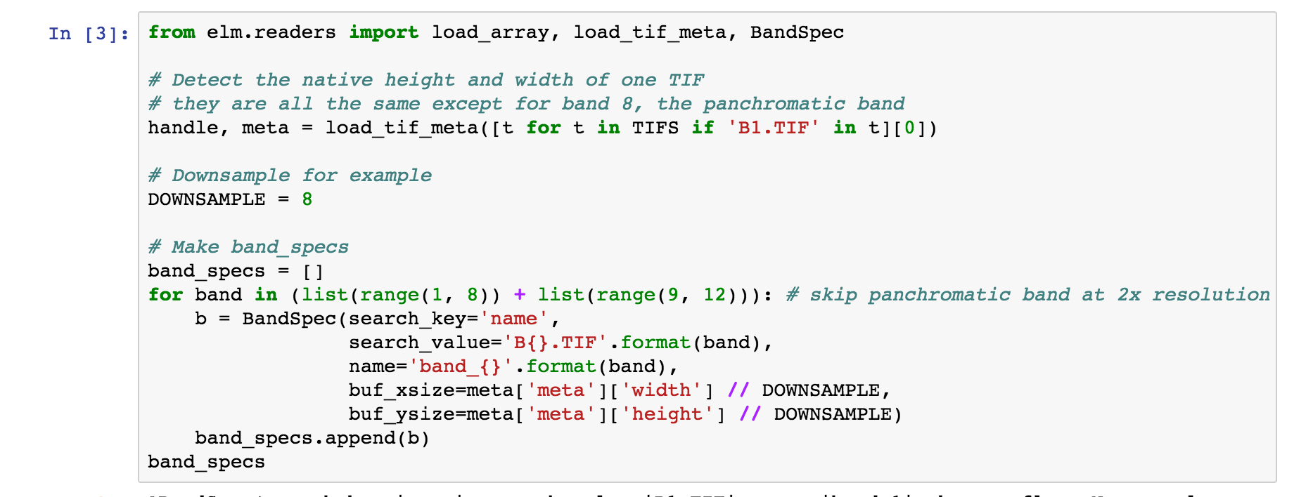
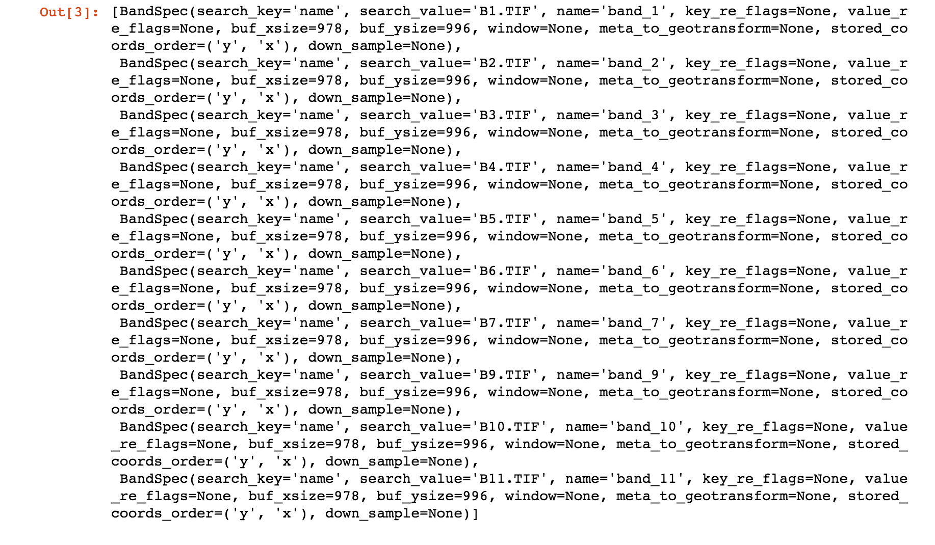
Check the repr of the BandSpec objects to see all possible arguments controlling reading of bands:

elm.readers.load_array

load_array aims to find a file reader for a NetCDF, HDF4, HDF5, or GeoTiff source.

The first argument to load_array is a directory if reading GeoTiff files and it is assumed that the directory contains GeoTiff files each with a 1-band raster.

For NetCDF, HDF4, and HDF5 the first argument is a single filename, and the bands are taken from the variables (NetCDF) or subdatasets (HDF4 / HDF5).

band_specs (list of BandSpec objects) is passed in to load_array (the list of BandSpec objects from above) to control which bands are read from the directory of GeoTiffs.

Using an ElmStore like an (xarray.Dataset)

See also xarray docs on Dataset

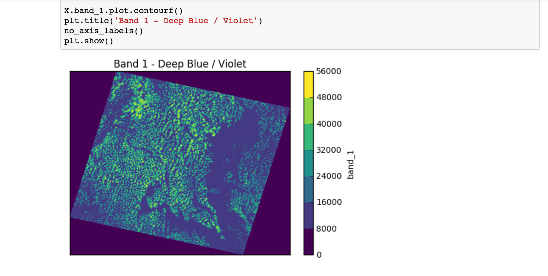
Visualization with ElmStore

The notebook then goes through a number of examples similar to:

• X.band_1.plot.pcolormesh() - The code uses names like band_1, band_2. These are named DataArray objects in the ElmStore X because of the name argument to the BandSpec objects above. The plot.pcolormesh() comes from the data viz tools with xarray.DataArray .
• The output of X.band_1.plot.pcolormesh()

Building a Pipeline

Building an elm.pipeline.Pipeline of transformations is similar to the idea of a Pipeline in scikit-learn.

• All steps but the last step in a Pipeline must be instances of classes from the elm.pipeline.steps - these are the transformers.
• The final step in a Pipeline should be an estimator from scikit-learn with a fit/predict interface.

The notebook shows how to specify a several-step Pipeline of

• Flattening rasters
• Assigning NaN where needed
• Dropping NaN rows
• Standardizing (Z-scoring) by band means and standard deviations
• Adding polynomial interaction terms of degree two
• Transforming with PCA
• K-Means with partial_fit several times per model

Preamble - Imports

This cell show typical import statments for working with a elm.pipeline.steps that become part of a Pipeline, including importing a transformer and estimator from scikit-learn:

Steps - Flatten

This transform-flatten step is essentially .ravel on each DataArray in X to create a single 2-D DataArray :

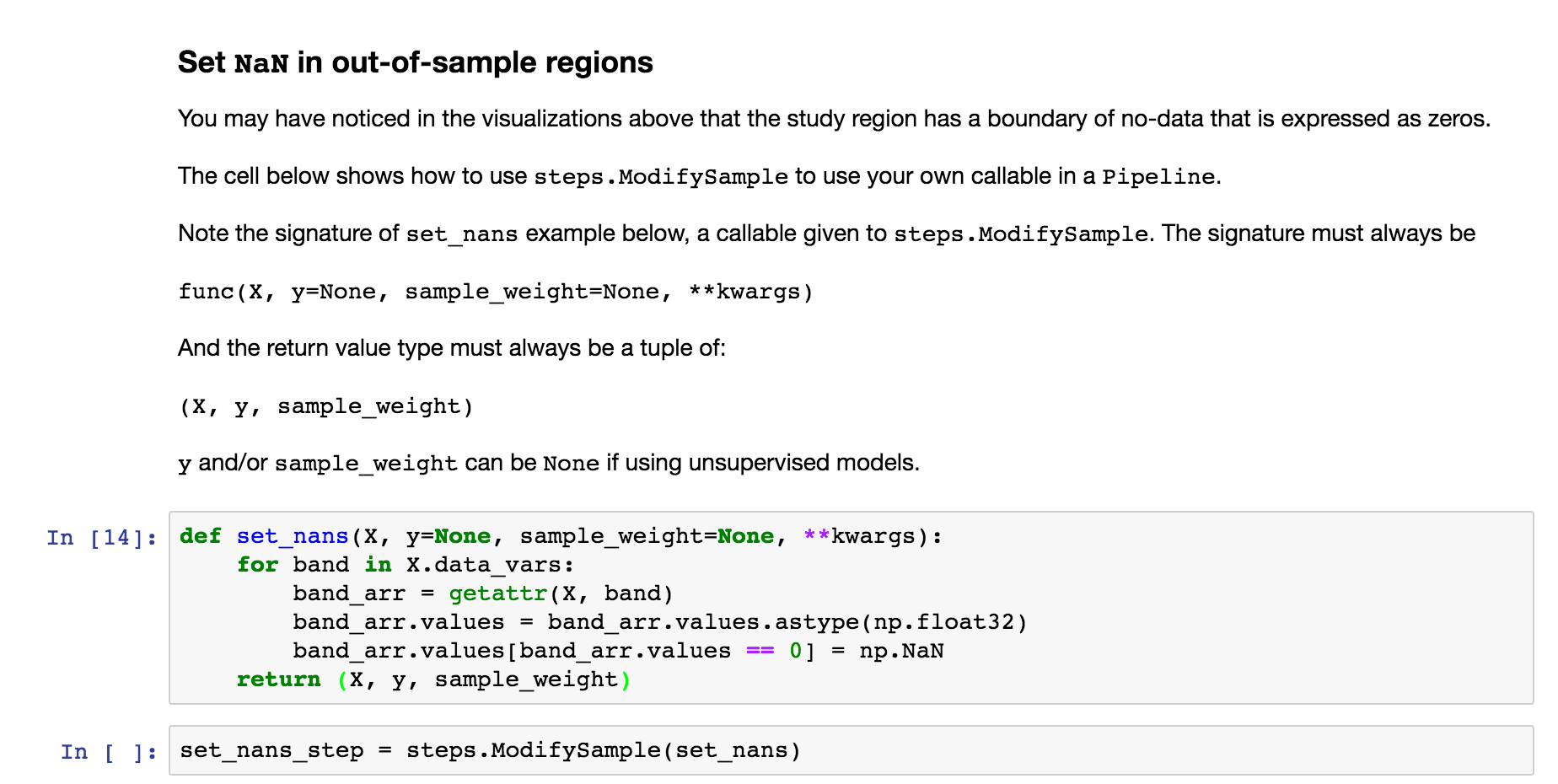
Steps - ModifySample - set_nans

The next step uses elm.pipeline.steps.ModifySample to run a custom callable in a Pipeline of transformations. This function sets NaN for the no-data perimeters of the rasters:

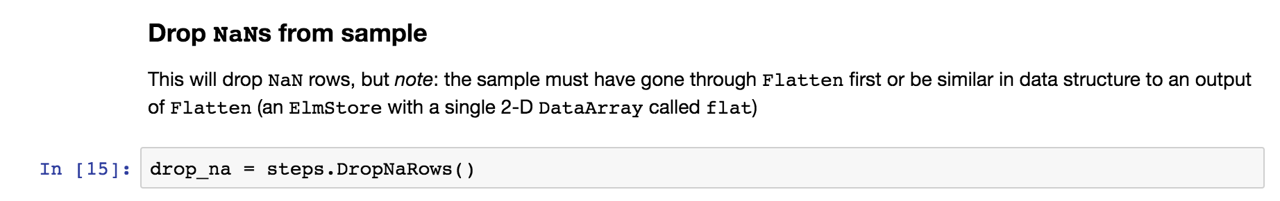
Steps - DropNaRows - Drop Null / NaN Rows

The transform-dropnarows is a transformer to remove the NaN values from the DataArray flat (the flattened (ravel) rasters as a single 2-D DataArray )

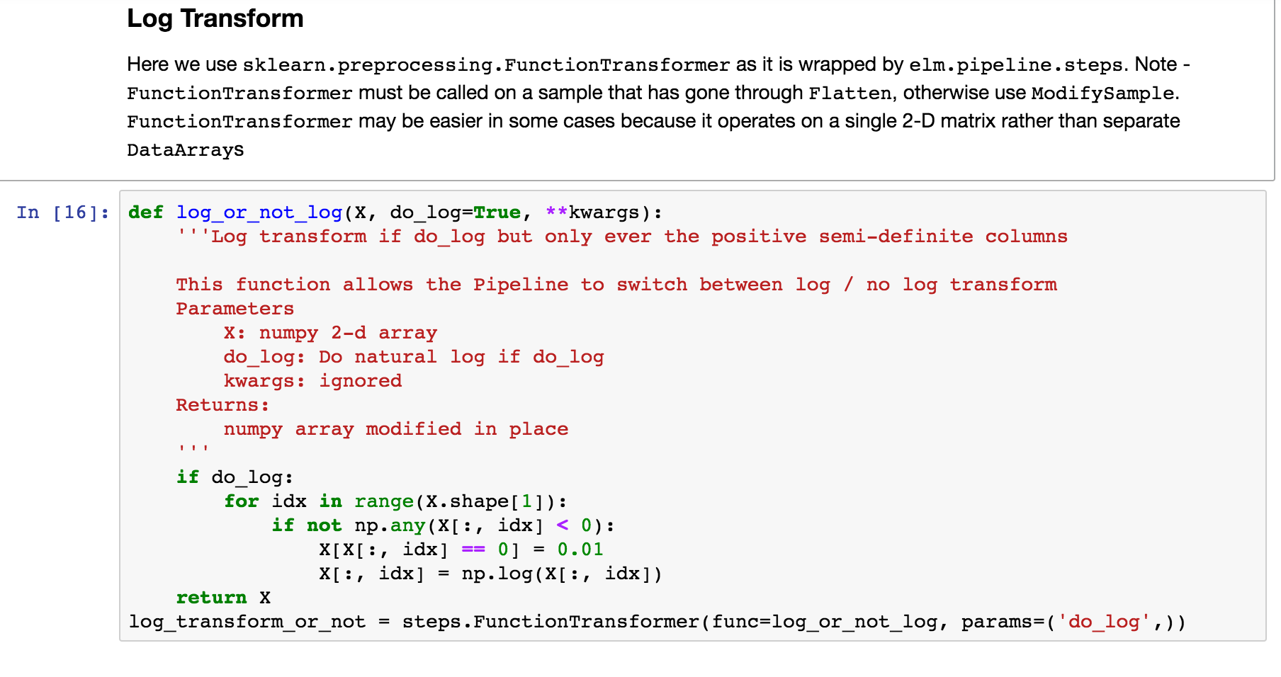
Steps - ModifySample - Log Transform (or pass through)

This usage of ModifySample will allow the Pipeline to use log transformation or not (see usage of set_params several screenshots later)

Feature engineering in a Pipeline

Define a function that can do normalized differences between bands (raster or DataArray ), adding the normalized differences to what will be the X data in the Pipeline of transformations.

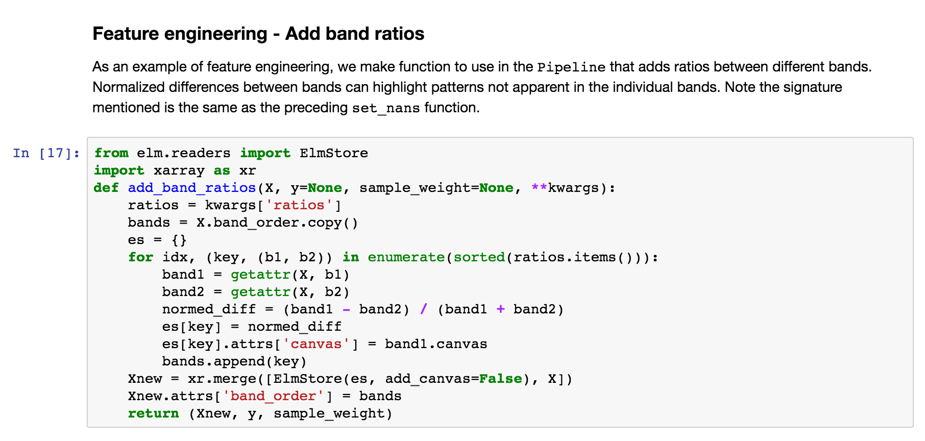
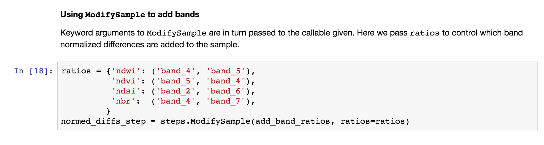
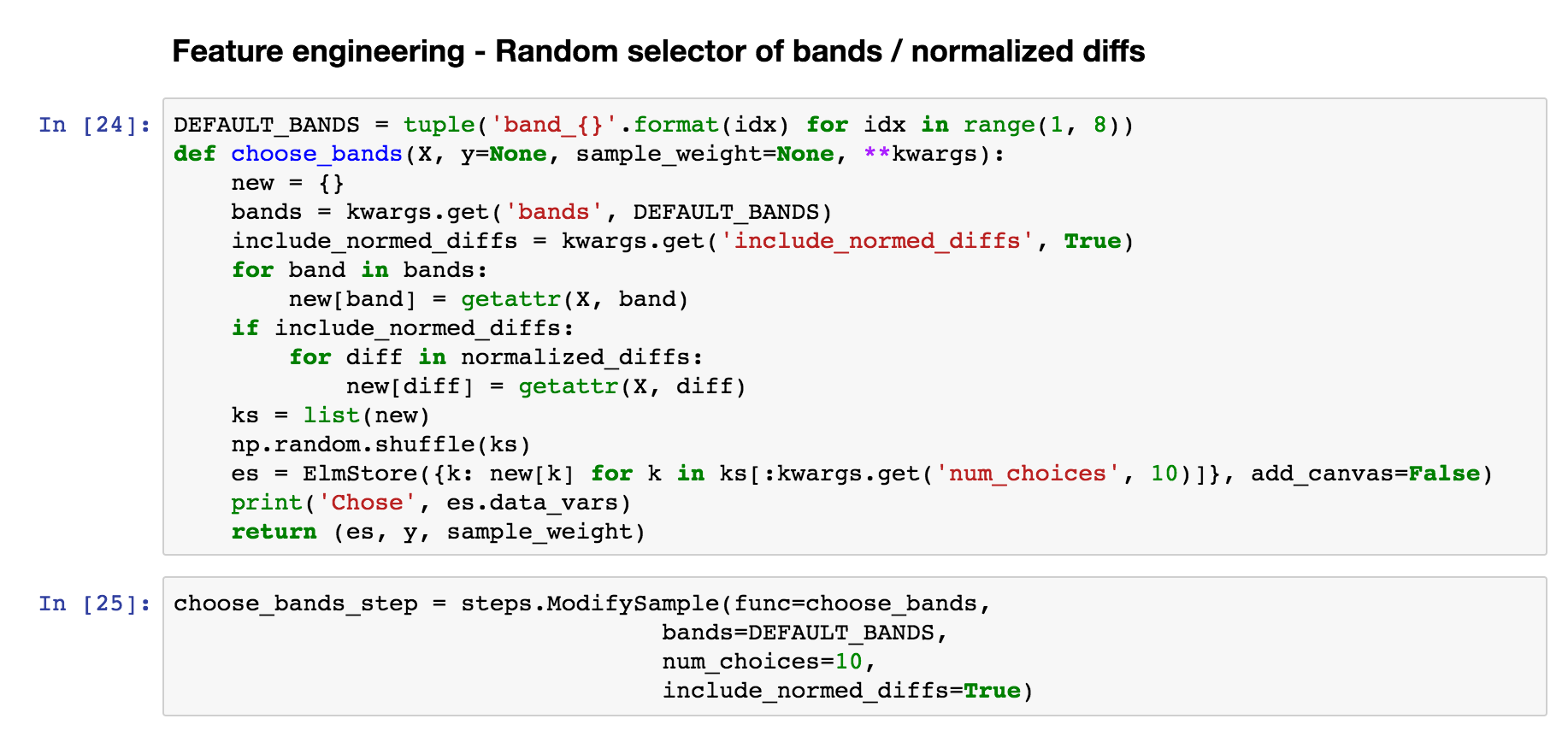
Feature engineering - ModifySample with arguments

And here is how the function above can be used in a Pipeline (wrapping with elm.pipeline.steps.ModifySample ):

We are calculating:

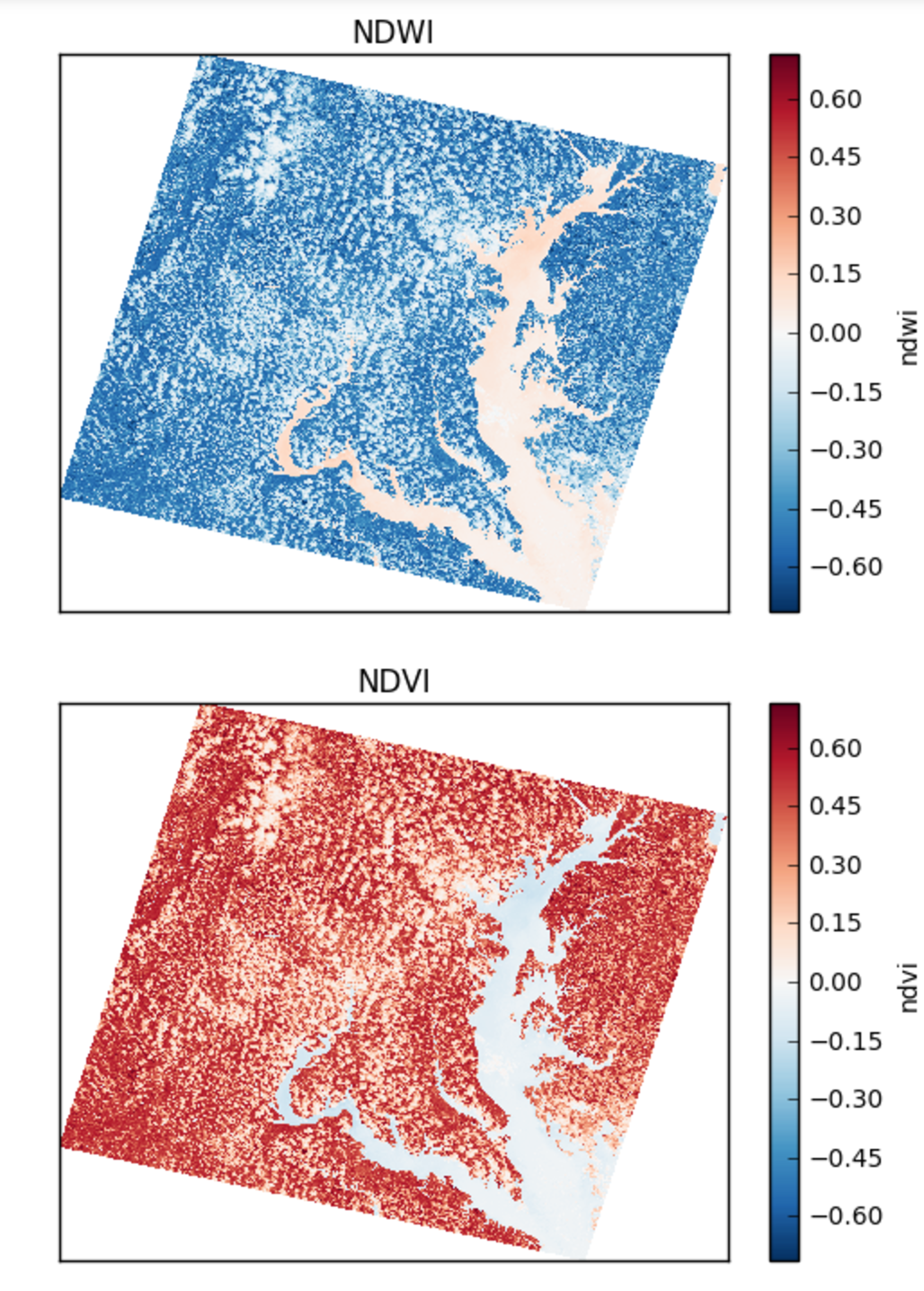
• NDWI : Normalized Difference Water Index * (band_4 - band_5) / (band_4 + band_5)
• NDVI : Normalized Difference Vegetation Index * (band_5 - band_4) / (band_5 + band_4)
• NDSI : Normalized Difference SnowIndex * (band_2 - band_6) / (band_2 + band_6)
• NBR : Normalized Burn Ratio * (band_4 - band_7) / (band_7 + band_4)

Using pcolormesh on normalized differences of bands

Here are the NDWI and NDVI plotted with the `xarray-pcolormesh`_ method of the predict DataArray

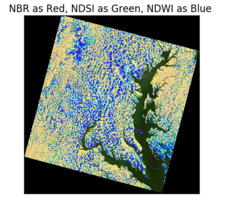
False Color with normalized differences of bands

The image below has an RGB (red, green, blue) matrix made up of the NBR , NDSI , NDWI normalized differences:

Normalization and Adding Polynomial Terms

The following snippets show how to use a class from sklearn.preprocessing or sklearn.feature_selection with Pipeline :

Custom Feature Selection

By defining the function below, we will be able to choose among random combinations of the original data or normalized differences

PCA

Use steps.Transform to wrap PCA or another method from sklearn.decomposition for elm.pipeline.Pipeline .

Read more on sklearn.decomposition models here.

Use an estimator from scikit-learn

Use a model with a fit / predict interface, such as KMeans.

Most scikit-learn models described here are supported.

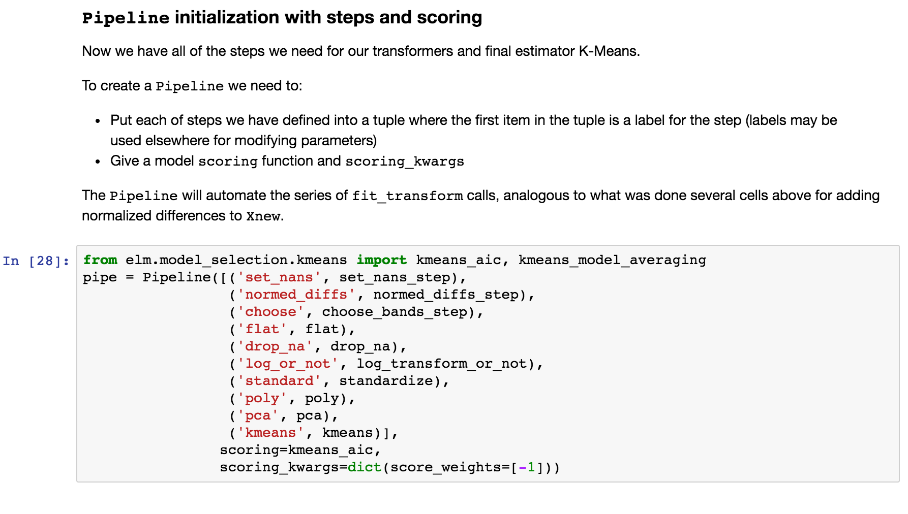
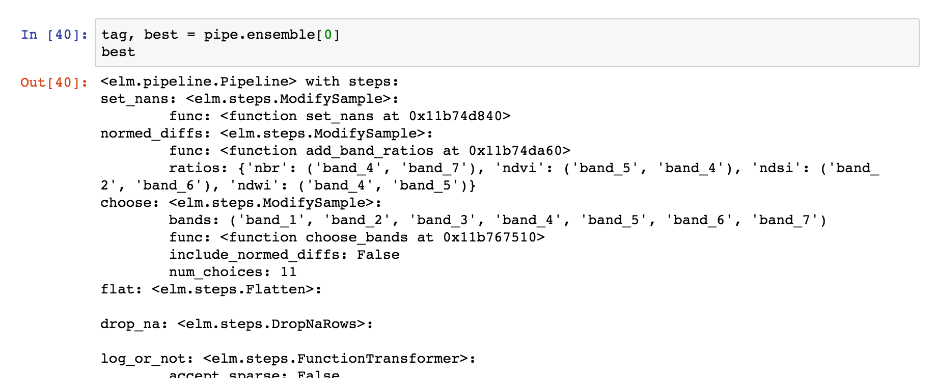
Create Pipeline instance

The following uses all the steps we have created in sequence of tuples and configures scoring for K-Means with the Akaike Information Criterion.

The next steps deal with controlling fit_ensemble (fitting with a group of models of different parameters)

See more info on Pipeline here.

ensemble_init_func

This is an example ensemble_init_func to pass to fit_ensemble, using pipe.new_with_params(**new_params) to create a new unfitted Pipeline instance with new parameters.

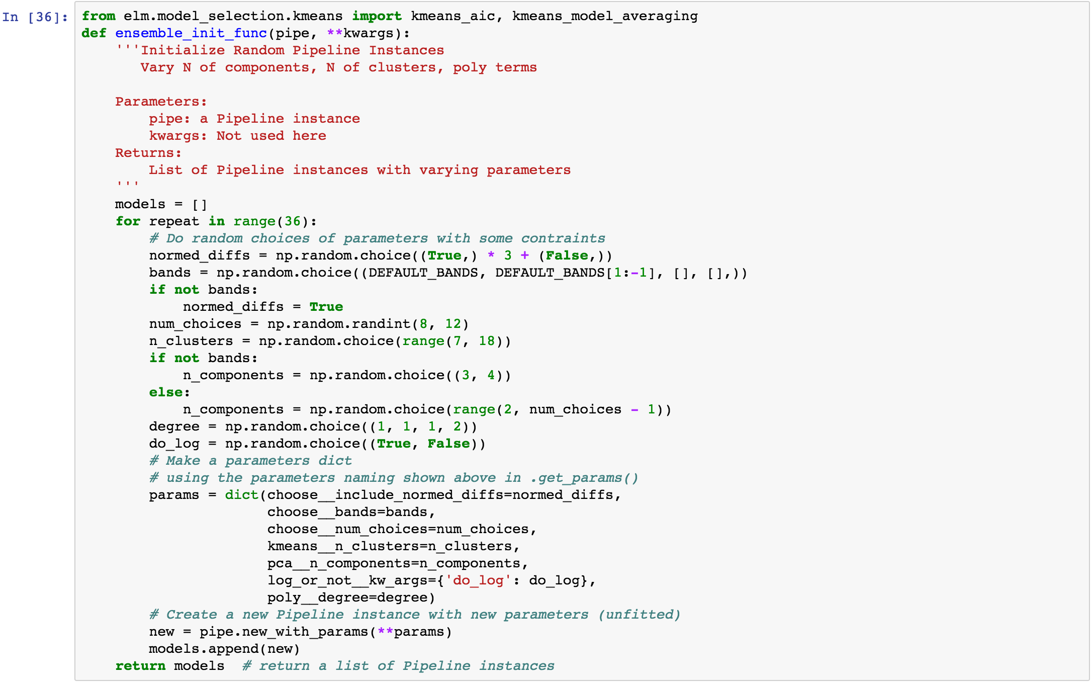
The fit_ensemble docs also show an example of an ensemble_init_func.

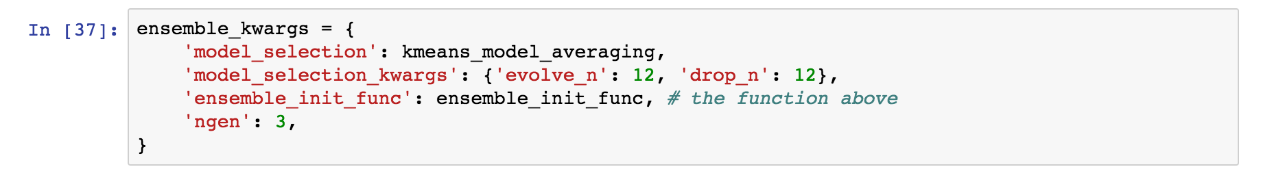
More fit_ensemble control

The following sets the number of generations ( ngen ) and the model_selection callable after each generation.

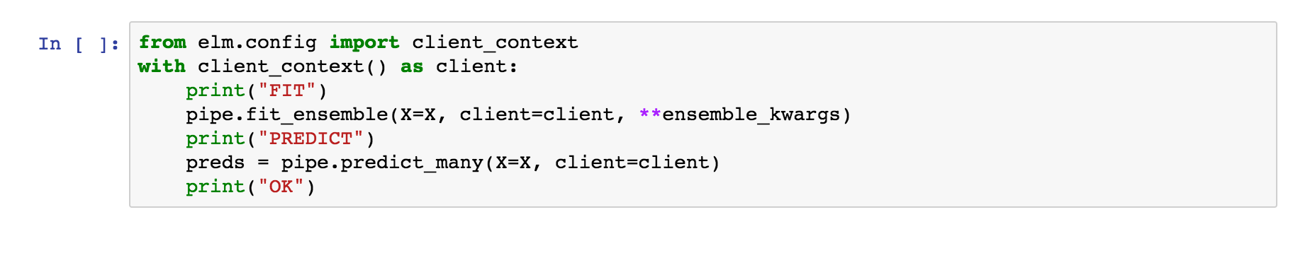
Parallelism with dask-distributed

fit_ensemble , to fit a group of models in generations with model selection after each generation, and predict_many each take a client keyword as a dask Client (dask). predict_many parallelizes over multiple models and samples, though here only one sample is used.

Using an ElmStore from predict_many

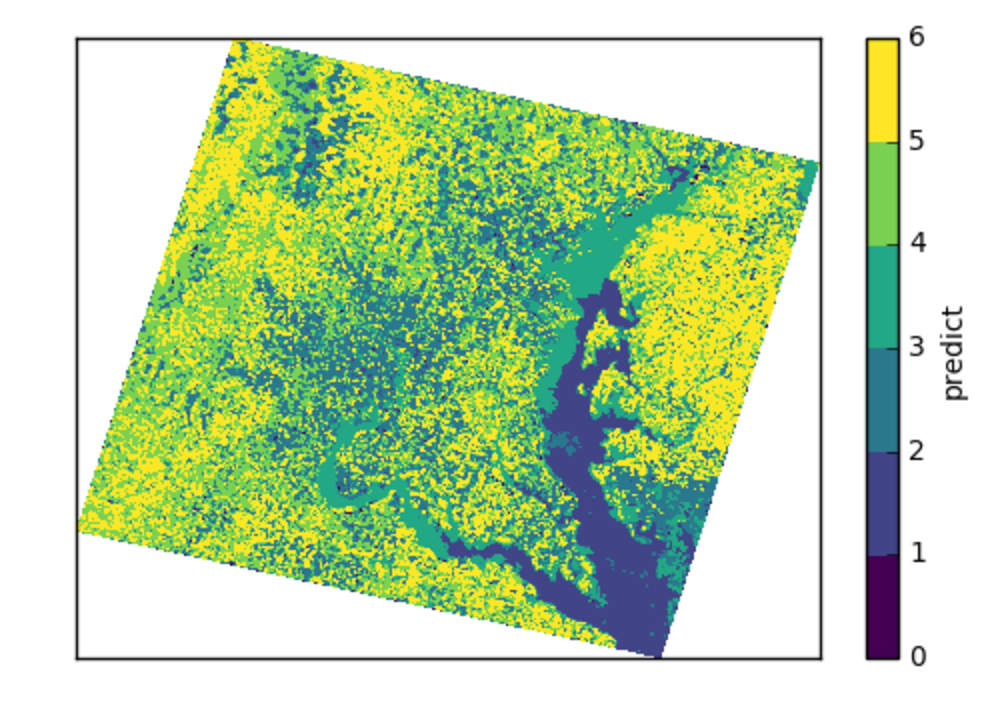
predict_many has called transform-inverseflatten to reshape the 1-D numpy array from the sklearn.cluster.KMeans.predict method to a 2-D raster with the coordinates of the original data. Note also the inverse_flatten is typically able to preserve NaN regions of the original data (the NaN borders of this image are preserved).

Using the xarray’s pcolormesh on the predict attribute ( DataArray ) of an ElmStore returned by predict_many :

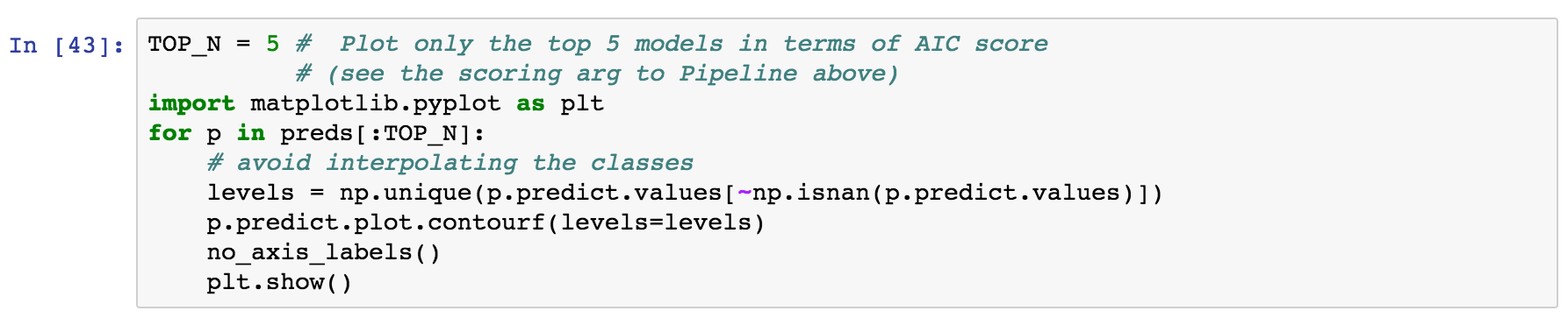
The best prediction in terms of AIC :